Optical Flow
1. Background
Optical flow is the approximated motion vector at each pixel location. It can tell us about the relative distances of objects, as closer moving objects will have more apparent motion than moving objects that are further away, given equal speed. The explanation on this page follows the treatment in [1].
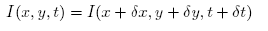
Optical flow is based on the assumptions that objects in the image at time t
will generally still be in the image at time t+1, only they will be displaced.
This is represented by
This leads via Taylor series expansion to the 2D motion constraint equation
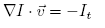
This one equation has two unknowns and so does not have a unique solution.
This is the mathematical consequence of the aperture problem. The aperture
problem is that there is not enough information in a small area to
uniquely determine motion (this is what causes the barber pole illusion).
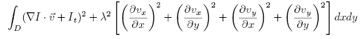
To add an additional constraint, Horn and Schunck [2] use
a global regularization calculation.
They assume that images consist of
objects undergoing rigid motion, and so over relatively large areas the
optical flow will be smooth. They then minimize the square of the
magnitude of the gradient of optical flow using the equation
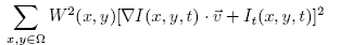
In contrast, Lucas and Kanade [3] use a local least squares calculation
to provide the constraint by minimizing in the neighborhood
surrounding the pixel, represented in equation form by
2. Implementation
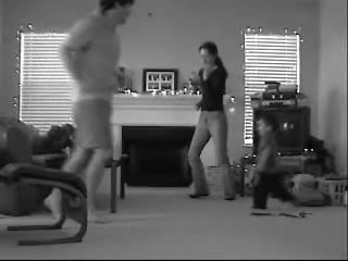
Given the image sequence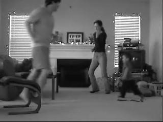
All partial derivatives were calculated as was outlined in [2].
The partial spatial derivative
in the x direction and the partial spatial derivative in the y direction
are shown here
and the partial derivative in time direction is shown here
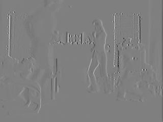
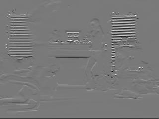
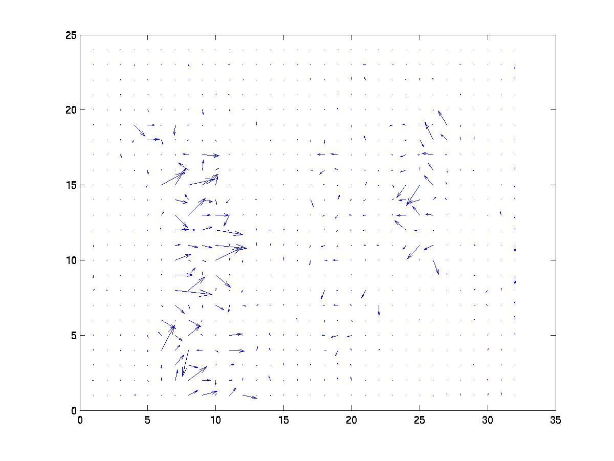
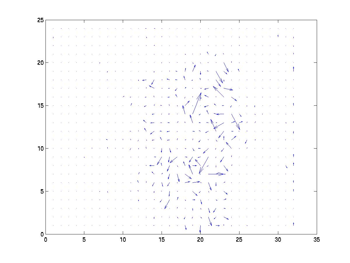
Using Horn and Schunck [2] the calculated optical flow for the
example images is
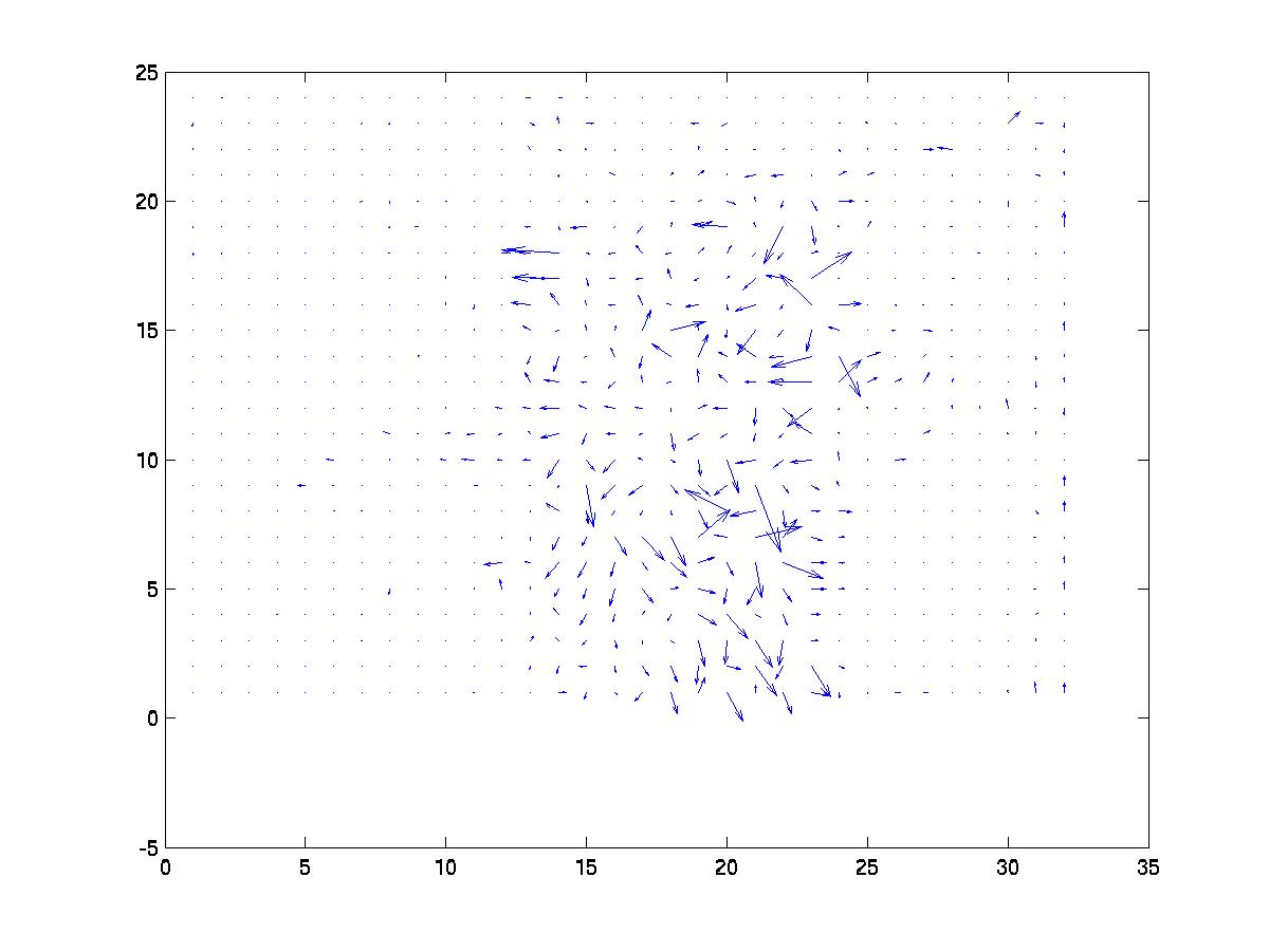
and using Lucas and Kanade [3] it is
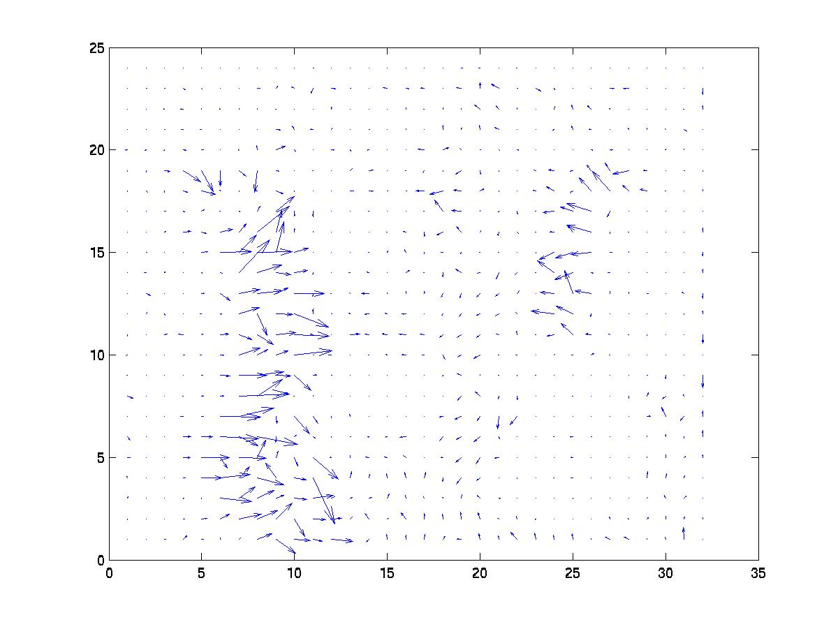
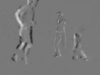
Both methods were able to identify me running from the left to
the right. My wife's movement was more subtle and that was represented
in the flow, however the movement of my son was not represented due to
his partial spatial derivatives being lost in the clutter of the television set.
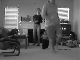
It did less well with movement towards the camera. Given the frames

Using Horn and Schunck [2] the calculated optical flow for the
example images is
and using Lucas and Kanade [3] it is
Here is a video (1.4 MB) of the optical flow calculated as in [2] from the movie in the discovering objects section of the project.
References
[1] J.L. Barron and N.A. Thacker, "Tutorial: Computing 2D and 3D Optical Flow",
Tina Memo No. 2004-012, 2005.
[2] B.K.P. Horn and B.G. Schunck, "Determining Optical Flow", Artificial Intelligence,
17, 1981, 185-204.
[3] B.D. Lucas and T. Kanade, "An Iterative Image Registration Technique with an
Application to Stereo Vision", DARPA Image Understanding Workshop, 1981, 121-130.
I wrote a book called The Curiosity Cycle: Preparing Your Child for the Ongoing Technological Explosion.